GROMACS Molecular Dynamics analysis
Hello everyone!
This past month I had to re-do some Molecular Dynamics (MD) analysis and, since before that, I spent a lot of time working with projects that were more Machine Learning related, I had to remember the best way to perform an MD analysis. That's why came to me the idea to write a quick tutorial to help future me (let's never forget to write tutorials!!) and to help anyone else that needs a head start on how to do MD analysis.
The objective of this tutorial is not to teach how to perform a MD simulation, for that I think that mdtutorials has excellent tutorials. By the way the simulation I am going to use as exemple here today I perfomed following the Tutorial 1: Lysozyme in Water. This simulations are being perfomed using WSL2 on Ubuntu 18.04 with GROMACS 2020.4.
Change on GROMACS version?
So, first of all, if you are doing the simulation on your computer and you are going to do the analysis with the same GROMACS version, you don't need to worry about version compatibility. But a lot of times, you are going to be doing simulations using a cluster, and if you have a different GROMACS version on your computer, you just need to update your .tpr file to your GROMACS version, using this command:
gmx grompp -f md.mdp -c md_0_1.pdb -p topol.top -o md_0_1_new.tpr
Problems on visualization? You may have a PBC situation...
To visualize the protein you may use PyMOL and for MD simulations you may use VMD, UCSF Chimera.
If in the process of visualization, your protein seems broken, fragmented or have residues stretched out, don't panic (not yet!). This could be a Periodic Boundary Condition situation. You may refer to some people describing this situation over here and here.
Example of necessary PBC processing
For me, this situation happened a lot when using VMD to visualize the MD simulation. I had a lot of problems to fit the trajectory to make the protein look whole again. To fit the protein you are going to have to use the "gmx trjconv" tool. Be aware that there is a lot of options to choose to fit the trajectory, I advise starting whith the following option:
gmx trjconv -s md_0_1.tpr -f md_0_1.xtc -o md_0_1_noPBC.xtc -pbc mol -center
choose option 1 (Protein) for centering and the option 0 (System) for output.
If this option doesn't work for you, I recommend messing around with the options on "gmx trjconv -h" and also some research may help to see which is specifically best for you system.
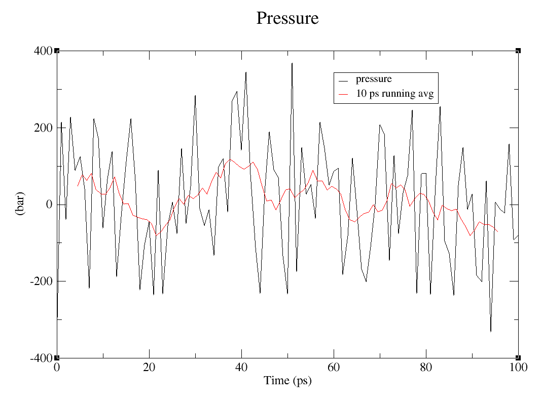
Energy minimization, temperature, density and pressure...
The calculation of this parameters are well explained in Tutorial 1: Lysozyme in Water, but one thing they don't explain clearly: How do they calculate the averages on the graphs?
I am going to use the QTGrace to plot all the graphs in this tutorial. Since it is not the scope of this tutorial to explain how to use QTGrace I am going to leave this tutorial, which cover the basics!
This step is also explained in the tutorial, but i thought it would be great to enphasize it here: Using the tool transform it is possible to run the averages. The number you are going to put on lenght of average depend on which average you wish to study, for me I stuck with 10 ps, so I selected 10 on lenght of average. And then, that is it! It was more simple than I expected it to be.
![]()
![]()
How to calculate averages on graph. First picture represent the first step, second picture the second step and last picture is how the graph should look like
Let's start the fun part... RMSD, RMSF, Rg?
This is how your movie simulation may be looking (visualization using UCSF Chimera, tutorial over here and here. In summary, to visualize the movie just go to tools>MD/Ensemble Analysis>MD Movie):
MD Simulation
To understand better how your system is behaving through the simulation it is important to analyze some properties of the dynamics: RMSD, RMSF, Rg. It is not the scope of this tutorial to explain this concepts, so feel free to read a bit about it and come back after understanding a little bit more.
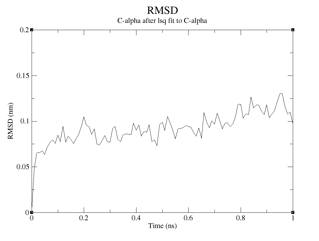
The RMSD diagram measures protein stability in the way that represents the spatial displacement rate and moving parts of the protein model during the simulation (SADR et al., 2021). By measuring the deviations it is possible to understand more about the structure stability. To calculate the RMSD of the protein, you are going to use the following command:
gmx rms -s md_0_1.tpr -f md_0_1_noPBC.xtc -o rmsd.xvg -tu ns
To calculate the RMSD of the crystal:
gmx rms -s em.tpr -f md_0_1_noPBC.xtc -o rmsd_xtal.xvg -tu ns
Which option you are going to choose between those two and between the options presented on group for least squares it and group or RMSD calculation, will depend on what kind of analysis you want to do. The RMSD of the system will be larger and will be interesting to analyze when you want to study the big picture. The RMSD of the c-alpha or the protein is the inverse.
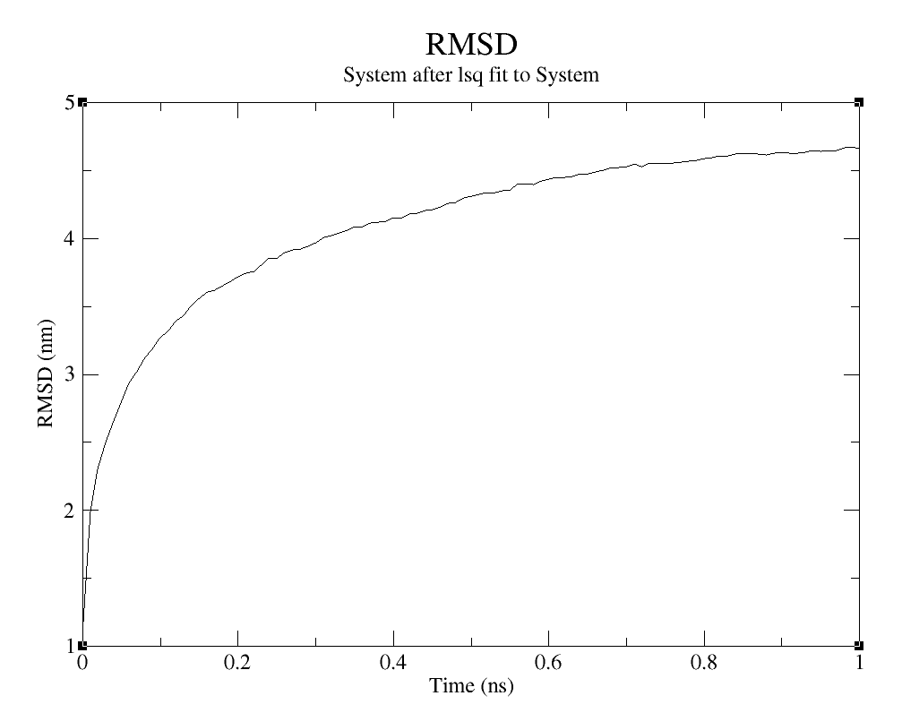
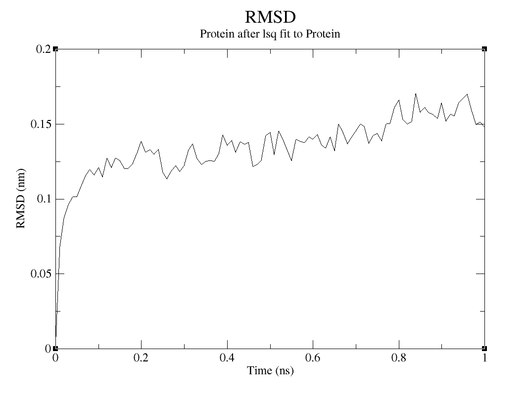
RMSD
Choose option 0 (System) group for least squares it and group and RMSD calculation to analyze the system, option 1 (Protein) or both to analyze protein and 3 (C-alpha) to analyze de C-alpha.
On the topic on how to evaluate this result, since the RMSD verifies the moving parts of the protein model, there is no huge displacement observed in the Protein and C-alpha graphs. But it is possible to assume that, the increase of simulation time is generating more movement on the model, which makes sense, since the residues are interacting with the water and ions on the simulation box.
To understand how each motion of Cα atoms reflects in the general motions of the structure, it is possible to investigate the structural fluctuation of the system by studying RMSF measurements. To calculate the RMSF for each atom, you re going to have to use the following command:
gmx rmsf -f md_0_1_noPBC.xtc -s md_0_1.tpr -o rmsf.xvg
But if you want to analyze the data by residue, you need to add the flag -res:
gmx rmsf -f md_0_1_noPBC.xtc -s md_0_1.tpr -o rmsf.xvg -res
As for the other analysis, you may to choose which group gmx will use to calculate de RMSF, in this tutorial I also choose C-alpha:
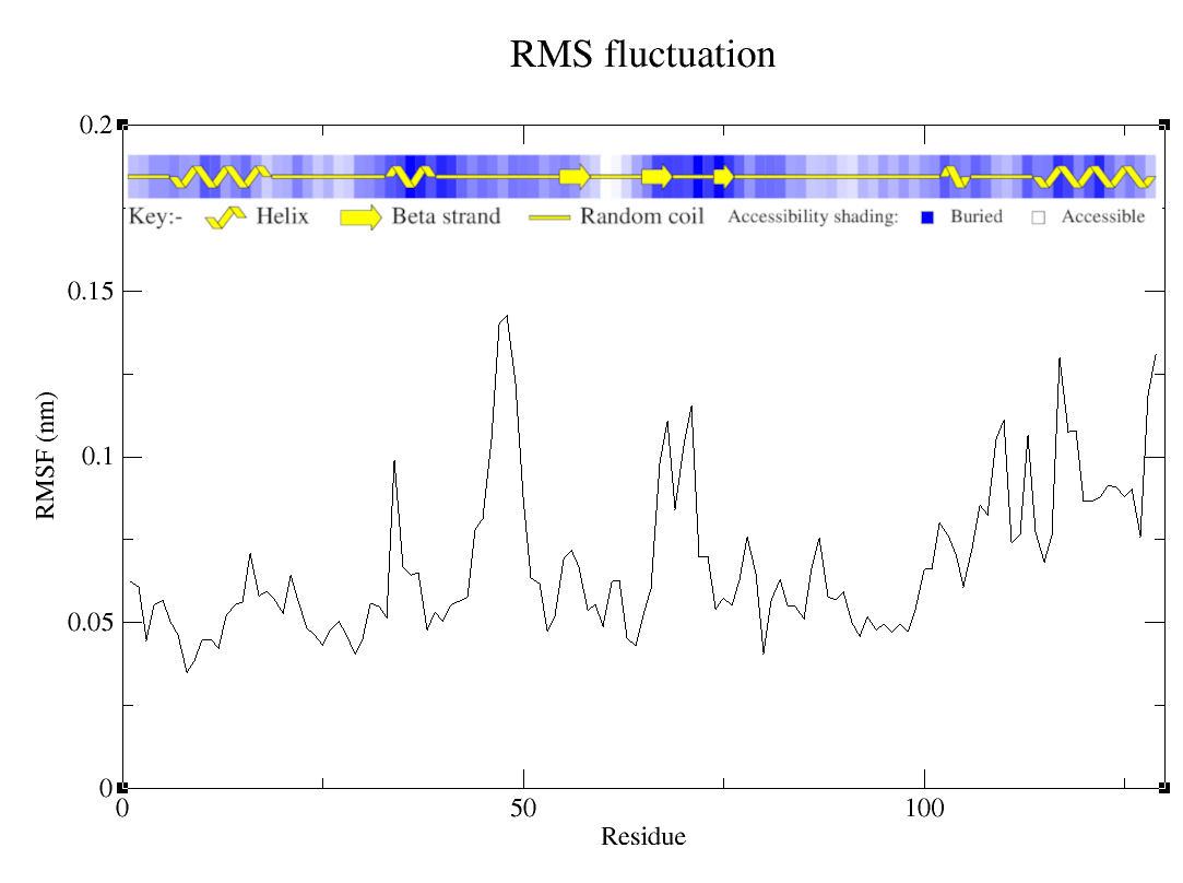
RMSF
The fluctuation by residue is intrisecally related to the topology of the protein. Which means, the more flexible the region, more it will fluctuate. In the case of the protein we simulated, the region around residues 45-50 are moving a lot, which makes sense, since it is in a loop region, naturally more flexible. The region towards the end of the protein is a helix-loop-helix region, which means it had to be a little bit more rigid. But we observe more flexibility in this region. This could mean that it is a region that should be more flexible because some catalytic activity or some mechanism that is related to the protein itself.
The Radius of gyration (Rg) is a measure of the stability of the protein after a MD simulation in a way that quantifies the deviation in the parameters in terms of compression and density. This is based on the principle that the more compact the protein is, the more stable it will be (LOBANOV et al., 2008). To calculate the Rg, you re going to have to use the following command:
gmx gyrate -s md_0_1.tpr -f md_0_1_noPBC.xtc -o gyrate.xvg
As for the other analysis, you may to choose which group gmx will use to calculate de Rg, in this tutorial I also choose C-alpha:
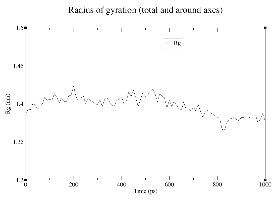
Rg
From this graph is possible to conclude that the protein is more compacted towards the end of the simulation, which means it is getting more and more stable.
How to represent my simulation on a frame?
When you want to save a moment in your life you take a picture, right? In this comparison, life is like a trajectory and a picture is used to get one moment of this trajectory and save. It is the same for the MD simulation, if you want to get the moment that most represent the MD movie you created in your simulation, you need to get the moment that most repeat itself and like in a picture you are going to get a frame of this movie.
To calculate the most representative moment of the MD simulation you need first to calculate the clusters of frames of the trajectory. For that you are going to use the following command:
gmx cluster -f md_0_1_noPBC.xtc -s md_0_1.tpr -cl md_0_1.pdb -g cluster.log
The file "cluster.log" has all the necessary information to analyze the clusters. In the table shown in the next figure, the important things to look for is: cl. represents the cluster number, #st represents the number of frames that are group in that cluster and middle rmsd, which is going to give to you the frame that is the median of all the clusters grouped in that group. In this case, the simulation could not generate clusters with more that one frame in each cluster, this could happen.
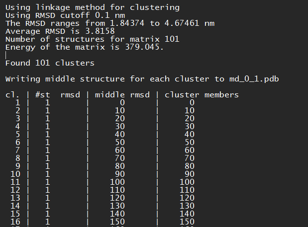
cluster.log example
So, I got another example here in the next picture. In this case, the cluster number 682 has 248 frames in which frame number 76930 is the median of all the frames grouped in this cluster. So, this is the one frame you are going to get to represent your simulation, if this cluster has the most amount of frames grouped in it. If another cluster has 300 frames, you are going to get the other one. Got it? Just look for the higher amount of frames in a cluster!
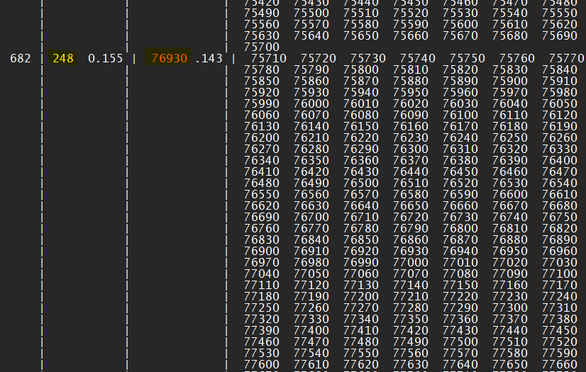
Another cluster.log example
In our case, since there is no most representative structure, I am going to analyze the first and the last frames of the simulation. To get the first frame you are going to use the following command:
gmx trjconv -s md_0_1.tpr -f md_0_1_noPBC.xtc -o start.pdb -dump 0
To get the last one:
gmx trjconv -s md_0_1.tpr -f md_0_1_noPBC.xtc -o end.pdb -dump 1000
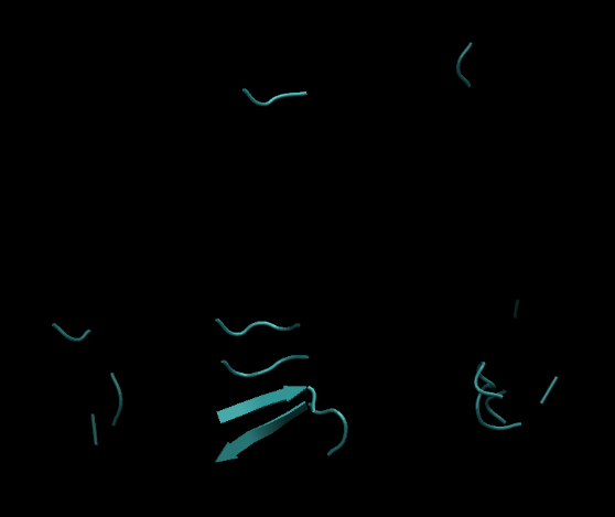
To visualize these structures I am going to use PyMOL (which I am going to leave a tutorial here). I am going to open both structures in the same window and use the PyMOL terminal to align the strucures using the following command:
align start, end
So, after that I get the following image:
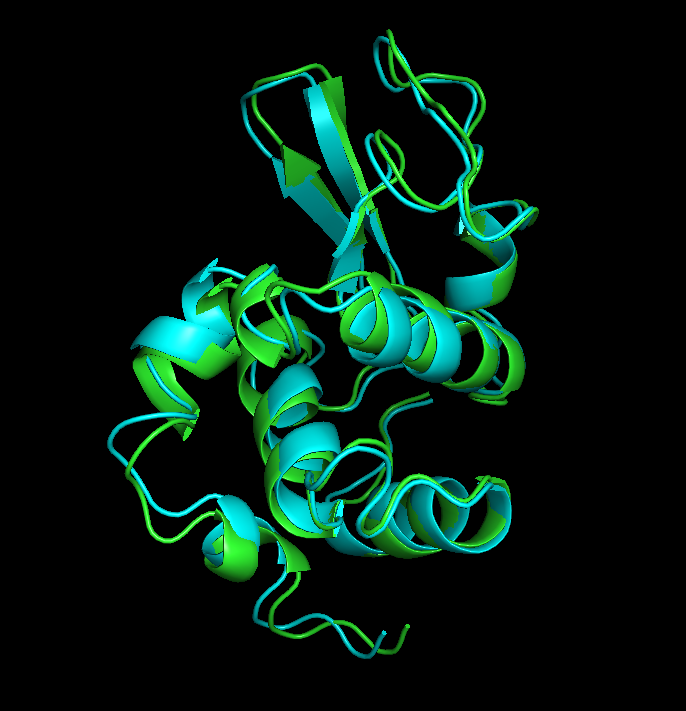
Start and end frames aligned
Since the time of simulation was only 1ns, no drastic changes were observed in the strucuture, which is shown by an RMSD of 1.088. It is possible to observe that, some loops are a little bit deslocated from its initial position and some alpha helices diminished in size. In simulations that run for a bigger amount of time it is possible to notice bigger changes.
So, that is it for the first part. This is only the basic stuff you could start with to analyze your MD simulation. Depending on which study you are going to perfom, other analysis could be useful, such as, PCA clustering, Ramachandran plots... between others. I am going to leave other tutorials here and here that could help. Feel free to ask anything on my LinkedIn page! (I will add a tool to ask questions here on the blog in the future)
I hope this tutorial was helpful for you as it was helpful for me doing it. Now, I am never going to skip the tutorial writing step!
References
LOBANOV, M. Yu; BOGATYREVA, N. S.; GALZITSKAYA, O. V. Radius of gyration as an indicator of protein structure compactness. Molecular Biology, v. 42, n. 4, p. 623-628, 2008.
SADR, Ahmad Shahir et al. In silico studies reveal structural deviations of mutant profilin-1 and interaction with riluzole and edaravone in amyotrophic lateral sclerosis. Scientific reports, v. 11, n. 1, p. 1-14, 2021.